Introduction

This package contains utilities to use Human Connectome Project (HCP) data and HCP-like data (e.g. obtained from legacy data using ciftify) as well as corresponding parcellations with nilearn and other Python tools.

The HCP data differs from conventional volumetric fMRI data which records the BOLD signal from each voxel in a 3D volume in that the signal from the cortical surface is treated as a folded two dimensional surface, and hence the data is associated with vertices of a predefined surface mesh, while the subcortical structures are described volumetrically using voxels.

The CIFTI (more precisely CIFTI-2) file format encompasses both the cortical 2D surface data as well as the subcortical volume data. However, only the voxels associated with relevant subcortical structures are kept. Thus these data are quite richly structured. Although the standard Python tools for dealing with fMRI data like nibabel can read both the CIFTI-2 files containing the fMRI signals and the GIFTI files containing the surface mesh definitions, there is not much that one could do further out-of-the-box, in particular visualization using nilearn or processing parcellated data using e.g. machine learning tools which work exclusively with numpy arrays. The goal of this package is to ease the interoperability of HCP data and these standard Python tools.

The utilities mainly deal with plotting surface data, accessing the predefined subcortical structures as well as using various parcellations and identifying connected components on the cortical surface. Various helper functions aid e.g. in mapping the HCP fMRI cortical data to surface vertices for visualization etc. The functions work directly with numpy arrays of shape Tx91282 or 91282 for fMRI data, with T being the number of time frames, while 91282 is the standard HCP dimensionality for the 3T cortical surface and subcortical data.

Installation

Make sure that you have the following packages installed (e.g. using miniconda)

nibabel, nilearn, numpy, scikit-learn, matplotlib, pandas, scipy

Then install with

pip install hcp_utils

upgrade with

pip install --upgrade hcp_utils

Usage

Here we assume that the commands will be run in a Jupyter notebook as this allows for rotating and scaling the 3D plots with your mouse.

Getting started

First import prerequisities.

import nibabel as nib
import nilearn.plotting as plotting
import numpy as np
import matplotlib.pyplot as plt
%matplotlib inline

Then import hcp_utils:

import hcp_utils as hcp

We use nibabel to load a CIFTI file with the fMRI time series. We also extract the fMRI time series to a numpy array.

img = nib.load('path/to/fMRI_data_file.dtseries.nii')
X = img.get_fdata()
X.shape     # e.g. (700, 91282)

which corresponds to 700 time-steps and 91282 grayordinates.

The CIFTI file format for HCP 3T data partitions the 91282 grayordinates into the left- and right- cortex as well as 19 subcortical regions. We can easily extract say the signal in the left hippocampus using hcp.struct

X_hipL = X[:, hcp.struct.hippocampus_left]
X_hipL.shape    # (700, 764)

The other available regions are

hcp.struct.keys()

dict_keys([‘cortex_left’, ‘cortex_right’, ‘cortex’, ‘subcortical’, ‘accumbens_left’, ‘accumbens_right’, ‘amygdala_left’, ‘amygdala_right’, ‘brainStem’, ‘caudate_left’, ‘caudate_right’, ‘cerebellum_left’, ‘cerebellum_right’, ‘diencephalon_left’, ‘diencephalon_right’, ‘hippocampus_left’, ‘hippocampus_right’, ‘pallidum_left’, ‘pallidum_right’, ‘putamen_left’, ‘putamen_right’, ‘thalamus_left’, ‘thalamus_right’])

For convenience we define a function which normalizes the data so that each grayordinate has zero (temporal) mean and unit standard deviation:

Xn = hcp.normalize(X)

Plotting

In order to plot the cortical surface data for the whole bran, one has to have the surface meshes appropriate for HCP data and combine the ones corresponding to the left and right hemispheres into a single mesh.

In addition, the HCP fMRI data are defined on a subset of the surface vertices (29696 out of 32492 for the left cortex and 29716 out of 32492 for the right cortex). Hence we have to construct an auxilliary array of size 32492 or 64984 with the fMRI data points inserted in appropriate places and a constant (zero by default) elsewhere. This is achieved by the cortex_data(arr, fill=0), left_cortex_data(arr, fill=0) and right_cortex_data(arr, fill=0) functions.

hcp_utils comes with preloaded surface meshes from the HCP S1200 group average data as well as the whole brain meshes composed of both the left and right meshes. In addition sulcal depth data is included for shading. These data are packaged in the following way:

hcp.mesh.keys()

dict_keys([‘white_left’, ‘white_right’, ‘white’, ‘midthickness_left’, ‘midthickness_right’, ‘midthickness’, ‘pial_left’, ‘pial_right’, ‘pial’, ‘inflated_left’, ‘inflated_right’, ‘inflated’, ‘very_inflated_left’, ‘very_inflated_right’, ‘very_inflated’, ‘flat_left’, ‘flat_right’, ‘flat’, ‘sphere_left’, ‘sphere_right’, ‘sphere’, ‘sulc’, ‘sulc_left’, ‘sulc_right’])

Here white is the top of white matter, pial is the surface of the brain, midthickness is halfway between them, while inflated and very_inflated are mostly useful for visualization. flat is a 2D flat representation.

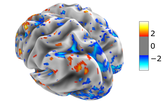
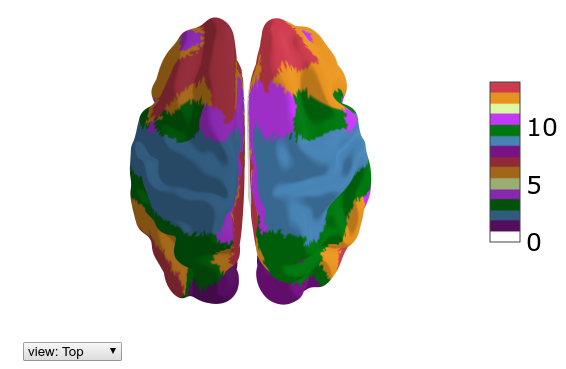
In order to make an interactive 3D surface plot using nilearn of the normalized fMRI data (thresholded at 1.5) at t=29 on the inflated group average mesh, we write

plotting.view_surf(hcp.mesh.inflated, hcp.cortex_data(Xn[29]), 
    threshold=1.5, bg_map=hcp.mesh.sulc)

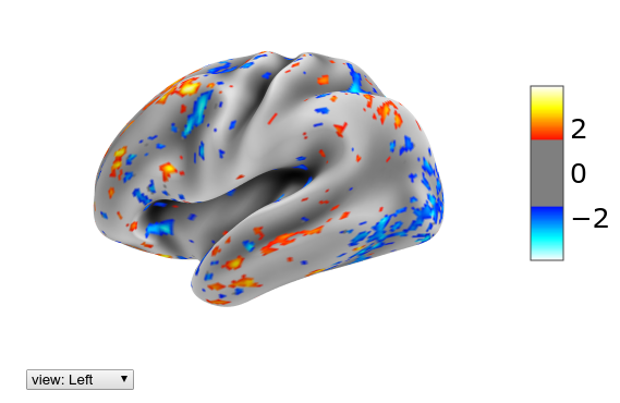
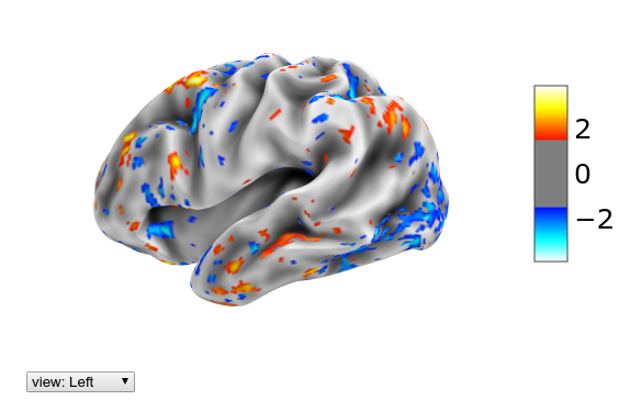
The group average surfaces are much smoother than the ones for individual subjects. If we have the latter ones at our disposal, we can also load them and use them for visualization.

mesh_sub = hcp.load_surfaces(example_filename='path/to/fsaverage_LR32k/
    sub-XX.R.pial.32k_fs_LR.surf.gii')

Here as an argument we give just one example filename and hcp_utils will try to load all other versions for both hemispheres and the sulcal depth file assuming HCP like naming conventions (the .R.pial part here).

Let’s look at the same data as previously, but now on the inflated single subject surface:

plotting.view_surf(mesh_sub.inflated, hcp.cortex_data(Xn[29]), 
    threshold=1.5, bg_map=mesh_sub.sulc)

Parcellations

hcp_utils comes with a couple of parcellations preloaded. In particular we have the following ones (where we also indicated the name of the variable with the parcellation data)

• the Glasser et.al. Multi-Modal Parcellation (MMP 1.0) which partitions each hemisphere of the cortex into 180 regions - hcp.mmp
• the Cole-Anticevic Brain-wide Network Partition (version 1.1) which
  • extends the Multi-Modal Parcellation of the cortex by a parcellation of the subcortical regions - hcp.ca_parcels
  • groups the cortical (MMP) and subcortical regions into functional networks - hcp.ca_network
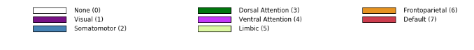
• the Yeo et.al. 7- and 17-region (cortical) functional networks - hcp.yeo7 and hcp.yeo17
• the standard CIFTI partition into the main subcortical regions - hcp.standard

For references and details see below or the github page. These parcellations were extracted from the relevant .dlabel.nii files by the scripts in the prepare/ folder of the package repository. Please cite the relevant papers if you make use of these parcellations.

All the labels and the corresponding numerical ids for these parcellations are displayed on the parcellation labels page.

The data for a parcellation contained e.g. in hcp.mmp has the following fields:

• parcellation.ids - numerical ids of the parcels. 0 means unassigned.
• parcellation.nontrivial_ids - same but with the unassigned one omitted.
• parcellation.labels - a dictionary which maps the numerical id to the name of the region
• parcellation.map_all - an integer array of size 91282, giving the id of each grayordinate
• parcellation.rgba - a dictionary which maps the numerical id to the rgba color (extracted from the source files)

One can view a cortical parcellation on the 3D surface plot using the following function

hcp.view_parcellation(mesh_sub.inflated, hcp.yeo7)

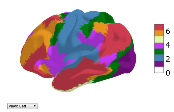
The color coding of the labels together with the numerical ids can be displayed through

hcp.parcellation_labels(hcp.yeo7)

Sometimes it may be convenient to differentiate between the networks in the left and right hemispheres. For that one can use the function make_lr_parcellation(parcellation) which takes a parcellation and separates the parcels in the left and right hemisphere. The subcortical part is set to zero (unassigned).

yeo7lr = hcp.make_lr_parcellation(hcp.yeo7)
hcp.view_parcellation(mesh_sub.inflated, yeo7lr)

hcp.parcellation_labels(yeo7lr)

The main use of a parcellation is to obtain the parcellated time series (by taking the mean over each parcel) for further analysis. This can be done through

Xp = hcp.parcellate(Xn, hcp.yeo7)
Xp.shape    # (700, 7)

One could e.g. take the maximum by writing instead

hcp.parcellate(Xn, hcp.yeo7, method=np.amax)

For visualization it might be interesting to plot the parcellated value on each location of the brain. For that we use the unparcellate(Xp, parcellation) function:

plotting.view_surf(mesh_sub.inflated, 
    hcp.cortex_data(hcp.unparcellate(Xp[29], hcp.yeo7)), 
    threshold=0.1, bg_map=mesh_sub.sulc)

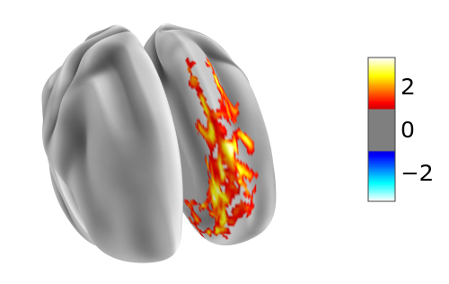
If we wanted to focus just on the activity in the somatomotor network of Yeo-7, we can mask out to 0 the remaining parts of the brain using mask(X, mask, fill=0). This is of course only useful for visualization:

plotting.view_surf(mesh_sub.inflated, 
    hcp.cortex_data(hcp.mask(Xn[29], hcp.yeo7.map_all==2)), 
    threshold=0.1, bg_map=mesh_sub.sulc)

Finally, once we have parcellated 1D data (e.g. a snapshot in time or the results of some analysis), we can order the regions according to the values using the function ranking(Xp, parcellation, descending=True):

df = hcp.ranking(Xp[29], hcp.yeo7)
df

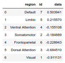
The above function returns a Pandas data frame which of course can be used for further analysis.

Connected components

Once some computation on the cortex data has been done and some boolean condition determined, it may be useful to decompose the region where the condition is satisfied into connected components.

cortical_adjacency is the 59412x59412 (sparse) adjacency matrix of the grayordinates on both hemispheres of the cortex.

The decomposition of the region where the boolean condition is satisfied into connected components is done by the function cortical_components(condition, cutoff=0) which returns the number of components, their sizes in descending order and an integer array with the labels of each grayordinate (0 means unassigned, labels ordered according to decreasing size of the connected components). If the cutoff parameter is specified, components smaller than the cutoff are neglected and the corresponding labels set to zero.

E.g. if we would insert a condition which is always true

n_components, sizes, rois = hcp.cortical_components(Xn[29]>-1000.0)
n_components, sizes

(2, array([29716, 29696]))

we would get just the two cortical hemispheres as the connected components.

A more realistic example would be

n_components, sizes, rois = hcp.cortical_components(Xn[29]>1.0, cutoff=36)
n_components, sizes

(42, array([1227, 415, 296, 276, 201, 168, 165, 143, 141, 115, 103, 101, 79, 77, 74, 69, 63, 62, 60, 52, 51, 51, 49, 48, 48, 45, 44, 43, 43, 43, 42, 40, 40, 39, 38, 38, 38, 38, 37, 37, 37, 36]))

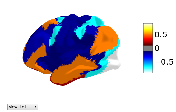
Then the largest connected component of size 1227 could be displayed by

plotting.view_surf(hcp.mesh.inflated, 
    hcp.cortex_data(hcp.mask(Xn[29], rois==1)), 
    threshold=1.0, bg_map=hcp.mesh.sulc)

External data and references

Surface meshes

The default surface meshes for 3D visualization come from the group average of the Human Connectome Project (HCP) 1200 Subjects (S1200) data release (March 2017) processed using HCP pipelines. They can be obtained on BALSA: https://balsa.wustl.edu/reference/show/pkXDZ

These group average files are redistributed under the HCP Open Access Data Use Terms with the acknowledgment:

“Data were provided [in part] by the Human Connectome Project, WU-Minn Consortium (Principal Investigators: David Van Essen and Kamil Ugurbil; 1U54MH091657) funded by the 16 NIH Institutes and Centers that support the NIH Blueprint for Neuroscience Research; and by the McDonnell Center for Systems Neuroscience at Washington University.”

Parcellations

When using the included parcellations, please cite the relevant papers, which include full details.

The Glasser MMP1.0 Parcellation: Glasser, Matthew F., Timothy S. Coalson, Emma C. Robinson, Carl D. Hacker, John Harwell, Essa Yacoub, Kamil Ugurbil, et al. 2016. “A Multi-Modal Parcellation of Human Cerebral Cortex.” Nature 536 (7615): 171–78. http://doi.org/10.1038/nature18933 (see in particular the details in Supplementary Neuroanatomical Results).

Yeo 7 or (17) Network Parcellation: Yeo, B. T. Thomas, Fenna M. Krienen, Jorge Sepulcre, Mert R. Sabuncu, Danial Lashkari, Marisa Hollinshead, Joshua L. Roffman, et al. 2011. “The Organization of the Human Cerebral Cortex Estimated by Intrinsic Functional Connectivity.” Journal of Neurophysiology 106 (3): 1125–65. https://doi.org/10.1152/jn.00338.2011.

The Cole-Anticevic Brain-wide Network Partition: Ji JL, Spronk M, Kulkarni K, Repovs G, Anticevic A, Cole MW (2019). “Mapping the human brain’s cortical-subcortical functional network organization”. NeuroImage. 185:35–57. https://doi.org/10.1016/j.neuroimage.2018.10.006 (also available as an open access bioRxiv preprint: http://doi.org/10.1101/206292) and https://github.com/ColeLab/ColeAnticevicNetPartition/

---

This package was initiated as a tool within the project “Bio-inspired artificial neural networks” funded by the Foundation for Polish Science (FNP).